
Diffusion Models for Molecule Design
“Creating noise from data is easy; creating data from noise is generative modelling.” — Yang Song


Introduction
Generative modelling, a technique that learns patterns in data to create new data, has experienced a renaissance in the past year. The catalyst was DALLE-2, an innovative image-to-text model revealed by the AI research firm OpenAI in April 2022. With DALLE-2, users can describe an image in plain text — encompassing multiple objects, scenes, or artistic styles — and the model will generate a brand new image from this description. The results have been noteworthy due to the extraordinary fidelity of the produced images and the model’s ability to seamlessly blend diverse abstract concepts within a single image. The model used a relatively new class of generative model called a diffusion model.

At this point, you might reasonably wonder, “What does this have to do with chemistry?”. Since DALLE-2, the buzz around ‘Generative AI’, a term seemingly coined by venture capitalists only recently, has since continued to intensify with many having found practical applications in the field of chemistry, particularly in the realm of drug discovery. By leveraging large datasets of chemical information, these AI models aim to generate new molecular structures with specific properties, offering a more targeted approach to drug development — at least in theory. It’s important to note that there are still challenges to overcome, such as the need for experimental validation and better evaluation altogether.
This article aims to simplify and summarize recent developments in generative models, specifically focusing on small molecule drug design using diffusion models. It takes a mostly technical approach, catering to readers without a background in machine learning. While briefly touching on challenges like data and evaluation, the main focus of this article is not on those aspects. For those interested in these perspectives and a broader commercial outlook, I highly recommend checking out Leonard Wossnig’s blog (CTO @ Labgenius). By exploring the unfolding story of diffusion models, this article aims to provide insights into current AI trends and their potential impact on the intersection of AI and (bio)chemistry.
What is Generative Modelling?

Generative modelling aims to learn from a dataset — be it images, text, music, or molecules — and replicate its underlying patterns to create new samples. By analysing a multitude of examples, the model discerns common features and characteristics, thereby understanding the distribution of different patterns within the dataset. Once the generative model has acquired knowledge about the distribution, it can generate new samples by sampling from this learned distribution. These generated samples are not simply copies of existing data points, but rather novel instances created based on the patterns and characteristics observed during training. This allows generative models to produce new and previously unseen samples that exhibit similar traits and qualities as the original data.
What are Diffusion Models?

Simply put, a diffusion model is a type of generative model that establishes a Markov chain of progressive noising, or ‘diffusion’ steps. In these steps, random Gaussian noise is added to real data until the original sample is unrecognisable. The next step is to train a model, typically a neural network, to reverse this process. Once trained, the model can create new samples by pulling from a normal distribution (random noise) and denoising this data until a high-quality, new sample emerges. That’s the fundamental idea, although be warned, a deeper understanding involves some equations.
Forward Diffusion Process
Suppose we have some real data (e.g. an image) that we call x₀, which is a sample from a true data distribution we wish to learn x₀~ p(x). We can define a forward diffusion process (q) which will gradually add a small amount of Gaussian Noise to the sample over T steps (where T is typically ~1,000), resulting in a sequence of progressively more noisy samples x₁, … , x_T. The amount of noise added at each step is controlled by a fixed variance schedule with, where will be between 0 and 1 depending on t.
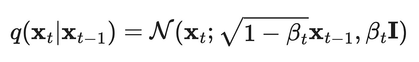
The sample x₀ will gradually lose its distinguishing features as t approaches T and the sample becomes fully noised, in other words, x_T is equivalent to a Gaussian distribution. We can say that q(xₜ|xₜ₋₁) represents the transitional probability distribution (i.e. the noise added) between xₜ₋₁ and xₜ.
Reverse (generative) diffusion process
We then teach a model to learn the reverse (or generative) diffusion process p_θ (xₜ₋₁ | xₜ) with tunable parameters θ, which will be able to generate new samples starting with some random data as input, x_T ~ 𝒩(0, I). Remember, while there is no information stored in a noisy image, there is information about how to make a new piece of data stored in the weights of the denoising model. More specifically, the model learns how to predict the mean and variance of the noise that was added to the data (although the variance is usually fixed in practice now).

To approximate the target denoising step p, it turns out that we only need to approximate the mean of the noise added to the data during the forward process ϵₜ, which is done using a denoising neural network ϵ_θ(xt, t). While the exact derivation of the training objective is complex, we can simplify by saying that our training objective is to minimise the difference between the true denoising process at every step t and the noise predicted by a tunable neural neural network ϵ_θ(xt, t), which takes as input the current noised sample xt and time step t.

Connection with score-based models
As is common in science, there were actually two different groups of people working on generative modelling that happened to arrive at the same formulation at similar times, approaching the problem from different perspectives. The first is the diffusion-based perspective which I’ve already described, and while the noise-denoise paradigm is good for a quick explanation, developing an intuitive understanding can be challenging. For those seeking a deeper understanding, I recommend exploring the second perspective, known as the score-based perspective.
In statistics, the score of a probability density function p(x) is defined as the gradient of the log of that function ∇ₓ log p(x). In score-based modelling, we aim to train a score network s_θ which tries to estimate the score such that s_θ(x) ≈ ∇ₓ log p(x). In generative modelling, we want to design a new sample x which has a high likelihood of being good quality according to the true data distribution p(x). By learning the gradient of p(x) with respect to x, the model essentially learns the direction in which x should be moved to improve its quality, that is, to increase its likelihood within the distribution. I would highly recommend this blog post by Yang Song for those interested in learning more.
Sampling with stochastic gradient Langevin dynamics
However, generating new data from a diffusion model (or score-based model) requires an additional trick to be effective. You can imagine that if you continue optimising a sample “x” solely based on the direction of a given score function, you will consistently converge to the same point on the learned distribution. This point typically corresponds to a mode within the training dataset, which, as you can imagine, is not particularly useful.
To address this issue, we draw inspiration from Langevin dynamics as commonly utilised in molecular dynamics simulations. In this approach, a small quantity of random noise is typically introduced to the simulation:

thus accounting for the impact of thermal fluctuations and interactions with the surrounding environment. By incorporating Langevin dynamics into our sampling process, we can obtain high-quality samples that are also diverse.
Diffusion models for molecule design
In the ensuing sections, I’ll be highlighting some notable works within the realm of diffusion models and generative chemistry. This overview will merely skim the surface of current developments, as 1–2 new papers on molecule generation using diffusion models emerge weekly. For those keen on staying abreast with the latest work, I recommend this continually updated list on GitHub. But before we delve in, let’s start with a brief history of molecule design through generative modelling.
Previously, deep generative models for small molecules typically fell into two categories: all-at-once and atom-by-atom generation. The former assumes atom independence during generation, which is unrealistic given molecule stability hinges on specific configurations. Conversely, atom-by-atom models necessitate an arbitrary atom ordering, complicating stable training.
Diffusion models present a compelling option for molecular design, utilising a process of iterative refinement. They gradually transform noise into molecules over several steps, enabling a methodical design process and the rectification of any errors along the way. This approach parallels the procedure employed by AlphaFold2’s Structure Module, which repeatedly refines its protein structure predictions through multiple model iterations until an accurate structure is achieved.
Equivariant Diffusion Model

Let’s begin our exploration of diffusion in generative chemistry by examining the well-known Equivariant Diffusion Model (EDM) paper. In this study, the authors trained a 3D diffusion model on a dataset composed of drug-like molecules to enable de novo generation of new molecules in 3D.
In this work, molecules are represented as graphs, where nodes are atoms and edges are chemical bonds, G = {N, E} with nodes N and edges E. Every node has two features z = [x, h], where h is a vector representing the atom type and x is another vector representing the coordinate. As in the above example with images, x and h can be viewed as such examples from the true data distribution to which we can add noise. They define a forward diffusion process q(zt|x,h), which gradually injects noise until the molecule becomes a blob of random atoms (see left of figure). Then train a reverse processp(zt-1|zt), which tries to predict the noise that was added to the data and then remove it to make clean data (see right of Figure).
As we represent molecules as graphs, is it very natural that we try to learn and reason over these graphs using Graph Neural Networks, a special kind of neural network that takes a graph (in this case molecule) as input, in order to predict the noise. As we are working with graphs that are in 3D, we use geometric GNNs which can handle these 3D features, which are technically equivalent GNNs. The word ‘equivariant’ simply means that we treat these graphs and the denoising process the same when the molecule is shifted and rotated in 3D space, the coordinate system in which we have the molecule is arbitrary. Figuring out which is the best equivariant GNN is a massive area of research and depends enormously on the exact problem you are working with in bio(chemistry).
DiffSBDD

This work was one of the first to introduce a DIFFusion model for Structure-based Drug Design (DiffSBDD), which recasts SBDD as learning to generate novel molecules conditional on a protein pocket structure. The model is built on top of the EDM framework but critically, the denoising networking takes as input the 3D structure of the target protein (which is represented as another 3D graph) as input, thus conditioning the generative procedure on the target structure.
DiffLinker is a similar method from the same group that is specifically designed for fragment linking within protein pockets. Here, they train a specialised model that takes a protein structure with fragments bound as inputs and generates a novel linker between them in 3D. They also have an additional auxiliary model, which predicts the size of the linker automatically.
DiffDock

DiffDock is a generative diffusion model, specialised for protein-ligand docking, not molecule design. It builds on the success of Torsion Diffusion, which excelled at generating molecular conformers by focusing on the molecule’s torsional angles while keeping bond length and angles constant — an excellent example of ‘inductive biases’ in machine learning. DiffDock was notable for recasting the docking problem as a generative one, rather than a predicting problem, as sampling from the model always gives a different pose (hopefully clustered around true binding modes).
What’s next for Diffusion Models in Chemistry?
As you might imagine, I’ve barely been able to scratch the surface of what is happening in diffusion modelling for chemistry currently. There is also an expansive literature applying these methods to de novo protein design as well. In my concluding section, I’d like to provide some commentary on three points: two challenges and one opportunity.
Data, data and data
As I said above, generative modelling is fundamentally based on learning the underlying distribution of a given dataset. Consequently, the quality and diversity of the training distribution significantly influence the performance and capabilities of the generative model. The model’s ability to generate samples that resemble the training data, capturing its patterns and characteristics, is limited by the training distribution itself. If the training distribution is of limited quality or lacks diversity, the generative model will be constrained and incapable of producing high-quality or novel samples beyond what it has learned.
This isn’t a problem if you are, say, trying to generate images of cats (the internet is very good for that sort of thing) but we very quickly run into problems when we start dealing with molecules. To give some perspective, for all its remarkable performance, DALLE-2 had to be trained on 400 million images from the internet, whereas, the number of high-quality protein-drug complexes we have available from the PDB is measured in the 10,000s, with the number of unique molecules and targets being even lower. People have tried to train on larger, synthetic datasets, produced by docking, but these of course come with their own sets of issues. Ultimately, this brings me back to the point that many people have made before, which is that we need more ‘machine learning-ready’ datasets if we want to solve a lot of these challenges.
More rigorous evaluations are needed
Unfortunately, machine learning publications live or die by their performance, with declarations of “state-of-the-art (SOTA) performance in [X]” almost a prerequisite for inclusion in top-tier machine learning conferences. This tendency, however, can unintentionally foster an environment of over-optimization towards simplified or flawed metrics, potentially guiding well-meaning computer scientists off course for considerable durations. The complexity of this issue escalates in fields like chemistry and drug discovery, where design processes are intricately multi-objective and abound with known unknowns.
For instance, DiffDock conducted a benchmark of their method against more conventional docking software, comparing the percentage of successful predictions with RMSD (Root Mean Square Deviation) less than 2 Å and the median RMSD. However, their evaluation was critised by some as it was performed in the blind docking scenario, where the binding site is unknown. In contrast, the methods they compared, such as Glide, are specifically designed for docking with known binding sites.
In February, a different group published an excellent benchmark paper that provided a fairer evaluation of these methods, by assessing both blind docking and docking with known pockets. The results indicated that traditional methods outperform DiffDock when docking into known pockets but that DiffDock excelled as a state-of-the-art binding site prediction algorithm, surpassing conventional methods. They suggested the optimal approach for blind docking is to first utilise DiffDock to detect the correct binding pocket and then employ conventional docking to achieve accurate positioning.
In my own field of SBDD with generative modelling, I’m worried we’re walking up a similar path. We’ve developed these 3D generative methods that generate a molecule and its pose simultaneously, ostensibly for efficiency — it’s quicker than generating the molecule first and then determining the pose through docking. Yet, when it comes to quality assessment, the focus tends to be solely on the molecules. Key metrics such as Quantitative Estimation of Drug-likeness (QED) and Synthetic Accessibility (SA) score are employed, but the assessment of the poses generated directly by the model is often overlooked, with molecules typically being redocked. This leaves a significant question unanswered: Are we truly creating models that excel at crafting high-affinity molecules with perfect protein-ligand complementarity? Or, in failing to assess pose quality, are we merely performing fancy atom filling with no concern to how the ligand interacts with the pocket? The distinction is critical, and it’s important to address this gap in our evaluation methods.
Other classes of generative models
Apart from diffusion models, the generative AI hype train has a few more carriages I’ve not had time to mention (some of which are actually worth paying attention to). One such model is GFlowNets, tailored specifically to maximise a certain ‘reward’ — like binding affinity, for instance. An intriguing ability comes from Large Language Models (LLMs) like GPT-4. While their primary function is to predict the next word, they can also generate novel molecules using SMILES strings. While I am personally sceptical, there are some serious people doing diligent research in this direction.
Conclusion
Generative modelling, through its capacity to understand and replicate the statistical properties of various datasets, has emerged as a potent tool for generating novel samples based on learned patterns and characteristics. Despite the potential, these models still face challenges, including data bias, data quality, and lack of rigorous evaluations being silent failures within the ML field. Overall, with the continual evolution of these models and advancements in computational capabilities, the impact of diffusion models in generative chemistry is expected to expand significantly in the coming years.
I would like to thank my colleagues at Cambridge, AstraZeneca, EPFL and Cornell for their insightful discussions that lead to many of the ideas explored in this article. I would also like to thank Leonard Wossnig, Helen Cooke and Chaitanya Joshi for their feedback on this blog. I would also like to thank my supervisors, Professors Pietro Lio and Sir Tom Blundell, for their guidance and support.
References
Ho, J., Jain, A. and Abbeel, P., 2020. Denoising diffusion probabilistic models. Advances in Neural Information Processing Systems, 33, pp.6840–6851.
Ramesh, A., Dhariwal, P., Nichol, A., Chu, C. and Chen, M., 2022. Hierarchical text-conditional image generation with clip latents. arXiv preprint arXiv:2204.06125.
Hoogeboom, E., Satorras, V.G., Vignac, C. and Welling, M., 2022, June. Equivariant diffusion for molecule generation in 3d. In International Conference on Machine Learning (pp. 8867–8887). PMLR.
Schneuing, A., Du, Y., Harris, C., Jamasb, A., Igashov, I., Du, W., Blundell, T., Lió, P., Gomes, C., Welling, M. and Bronstein, M., 2022. Structure-based drug design with equivariant diffusion models. arXiv preprint arXiv:2210.13695.
Corso, G., Stärk, H., Jing, B., Barzilay, R. and Jaakkola, T., 2022. Diffdock: Diffusion steps, twists, and turns for molecular docking. arXiv preprint arXiv:2210.01776.